Multisector modelling with Macro
The interactive version of this tutorial can be found here.
In this tutorial, we extend the electricity-only model considered in Tutorial 1 to build a multisector model for joint capacity expansion in electricity and hydrogen sectors.
To do this, we incorporate hydrogen and electricity demand from Tutorial 1, and endogenously model hydrogen production and storage in Macro.
using Pkg; Pkg.add(["VegaLite", "Plots"])using MacroEnergy
using HiGHS
using CSV
using DataFrames
using JSON3
using Plots
using VegaLiteCreate a new case folder named "one_zone_multisector"
if !isdir("one_zone_multisector")
    mkdir("one_zone_multisector")
    cp("one_zone_electricity_only/assets","one_zone_multisector/assets", force=true)
    cp("one_zone_electricity_only/settings","one_zone_multisector/settings", force=true)
    cp("one_zone_electricity_only/system","one_zone_multisector/system", force=true)
    cp("one_zone_electricity_only/system_data.json","one_zone_multisector/system_data.json", force=true)
end
Note: If you have previously run Tutorial 1, make sure that file one_zone_multisector/system/nodes.json is restored to the original version with a $\text{CO}_2$ price. The definition of the $\text{CO}_2$ node should look like this:
{
    "type": "CO2",
    "global_data": {
        "time_interval": "CO2"
    },
    "instance_data": [
        {
            "id": "co2_sink",
            "constraints": {
                "CO2CapConstraint": true
            },
            "rhs_policy": {
                "CO2CapConstraint": 0
            },
            "price_unmet_policy":{
                "CO2CapConstraint": 200
            }
        }
    ]
}
Add Hydrogen to the list of modeled commodities, modifying file one_zone_multisector/system/commodities.json:
new_macro_commodities = Dict("commodities"=> ["Electricity", "NaturalGas", "CO2", "Hydrogen"])

open("one_zone_multisector/system/commodities.json", "w") do io
    JSON3.pretty(io, new_macro_commodities)
end
Update file one_zone_multisector/system/time_data.json accordingly:
new_time_data = Dict(
    "HoursPerTimeStep" => Dict(
        "Electricity"=>1,
        "NaturalGas"=> 1,
        "CO2"=> 1,
        "Hydrogen"=>1
    ),
    "HoursPerSubperiod" => Dict(
        "Electricity"=>8760,
        "NaturalGas"=> 8760,
        "CO2"=> 8760,
        "Hydrogen"=>8760
    ),
    "NumberOfSubperiods"=>1,
    "TotalHoursModeled"=>8760
)

open("one_zone_multisector/system/time_data.json", "w") do io
    JSON3.pretty(io, new_time_data)
end
Move separate electricity and hydrogen demand timeseries into the system folder
cp("demand_timeseries/electricity_demand.csv","one_zone_multisector/system/demand.csv"; force=true)cp("demand_timeseries/hydrogen_demand.csv","one_zone_multisector/system/hydrogen_demand.csv"; force=true)Exercise 1
Using the existing electricity nodes in one_zone_multisector/system/nodes.json as template, add a Hydrogen demand node, linking it to the hydrogen_demand.csv timeseries.
Solution
The definition of the new Hydrogen node in one_zone_multisector/system/nodes.json should look like this:
{
    "type": "Hydrogen",
    "global_data": {
        "time_interval": "Hydrogen",
        "constraints": {
            "BalanceConstraint": true
        }
    },
    "instance_data": [
        {
            "id": "h2_NE",
            "location": "NE",
            "demand": {
                "timeseries": {
                    "path": "system/hydrogen_demand.csv",
                    "header": "Demand_H2_z1"
                }
            }
        }
    ]
},
Next, add an electrolyzer asset represented in Macro as a transformation connecting electricity and hydrogen nodes:
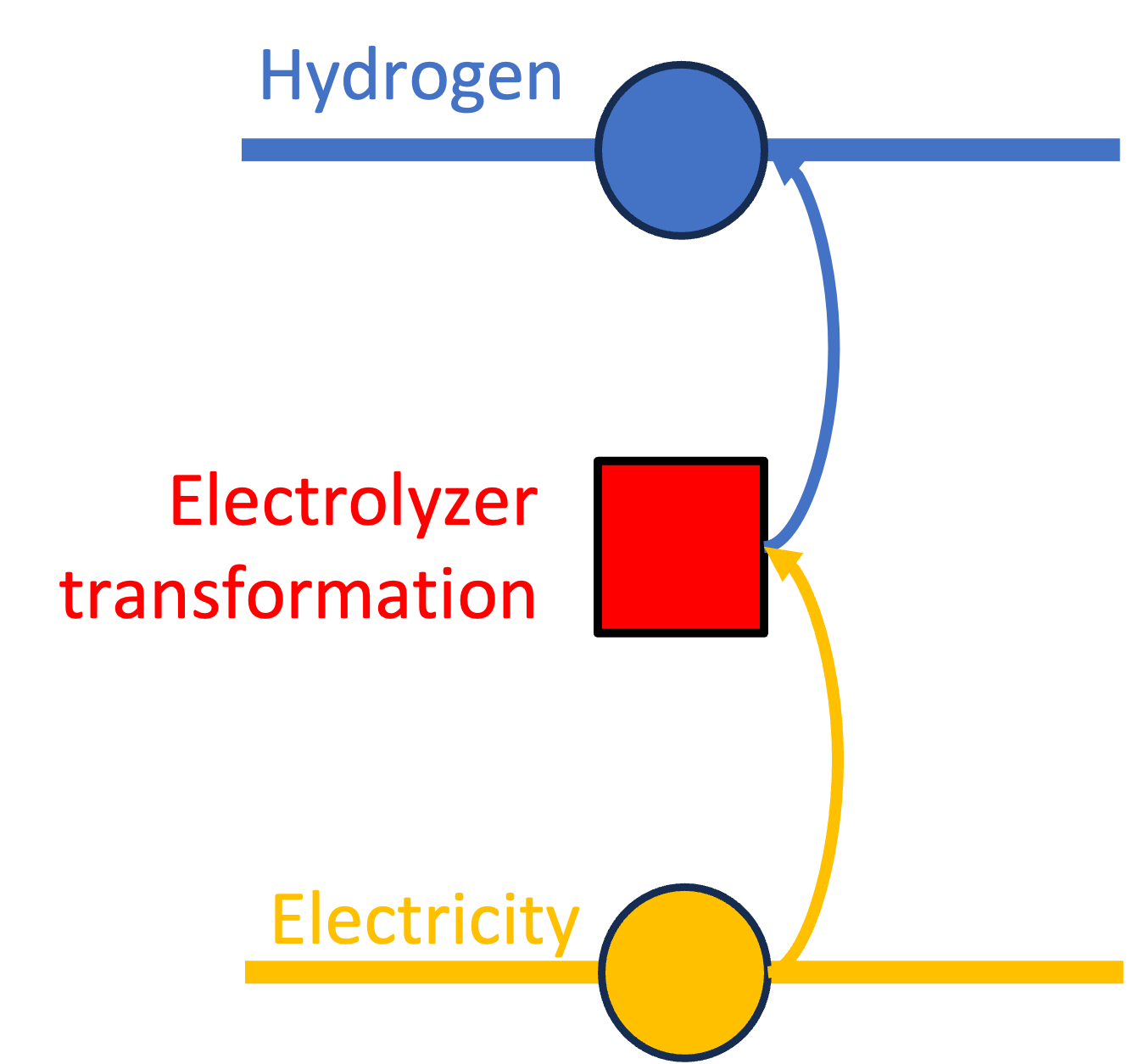
To include the electrolyzer, create a file one_zone_multisector/assets/electrolyzer.json based on the asset definition in src/model/assets/electrolyzer.jl:
{
    "electrolyzer": [
        {
            "type": "Electrolyzer",
            "instance_data": [
                {
                    "id": "NE_Electrolyzer",
                    "location": "NE",
                    "h2_constraints": {
                        "CapacityConstraint": true,
                        "RampingLimitConstraint": true,
                        "MinFlowConstraint": true
                    },
                    "efficiency_rate": 0.875111139,
                    "investment_cost": 41112.53426,
                    "fixed_om_cost": 1052.480877,
                    "variable_om_cost": 0.0,
                    "capacity_size": 1.5752,
                    "ramp_up_fraction": 1,
                    "ramp_down_fraction": 1,
                    "min_flow_fraction": 0.1
                }
            ]
        }
    ]
}
Include a hydrogen storage resource cluster, represented in Macro as combination of a compressor transformation (consuming electricity to compress the gas) and a storage node:
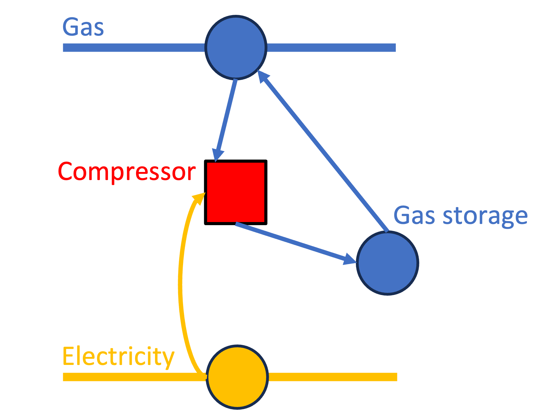
Add a file one_zone_multisector/assets/h2_storage.json based on the asset definition in src/model/assets/gasstorage.jl that should look like this:
{
    "h2stor": [
        {
            "type": "GasStorage",
            "instance_data": [
                {
                    "id": "NE_Above_ground_storage",
                    "location": "NE",
                    "storage_commodity": "Hydrogen",
                    "storage_can_retire": false,
                    "storage_investment_cost": 873.013307,
                    "storage_fixed_om_cost": 28.75810056,
                    "storage_loss_fraction": 0.0,
                    "storage_min_storage_level": 0.3,
                    "storage_constraints": {
                        "StorageCapacityConstraint": true,
                        "BalanceConstraint": true,
                        "MinStorageLevelConstraint": true
                    },
                    "discharge_can_expand": true,
                    "discharge_has_capacity": true,
                    "discharge_constraints": {
                        "CapacityConstraint": true,
                        "RampingLimitConstraint": true
                    },
                    "discharge_electricity_consumption": 0.018029457,
                    "charge_investment_cost": 3219.24,
                    "charge_efficiency": 1.0,
                    "charge_electricity_consumption": 0.018029457
                }
            ]
        }
    ]
}
Exercise 2
Following the same steps taken in Tutorial 1, load the input files, generate the model, and solve it using the open-source solver HiGHS.
Solution
First, load the inputs:
case = load_case("one_zone_multisector");Then, create the optimizer and solve the model:
optimizer = create_optimizer(HiGHS.Optimizer);
(case, solution) = solve_case(case, optimizer);
Exercise 3
As in Tutorial 1, print optimized capacity for each asset, the system total cost, and the total emissions.
What do you observe?
To explain the results, plot both the electricity generation and hydrogen supply results as done in Tutorial 1 using VegaLite.jl.
Solution
As in the previous tutorial, optimized capacities are retrieved as follows:
period_index = 1 # only one investment period in this example
system = case.systems[period_index];
columns_to_keep = [:commodity, :resource_id, :type, :value];
capacity_results = get_optimal_capacity(system);
capacity_results[:, columns_to_keep]new_capacity_results = get_optimal_new_capacity(system);
new_capacity_results[:, columns_to_keep]retired_capacity_results = get_optimal_retired_capacity(system);
retired_capacity_results[:, columns_to_keep]Total system cost is:
MacroEnergy.objective_value(solution)Total $\text{CO}_2$ emissions are:
co2_node = MacroEnergy.find_node(system.locations, :co2_sink);
MacroEnergy.value.(sum(MacroEnergy.get_balance(co2_node, :emissions)))
Note that we have achieved lower costs and emissions when able to co-optimize capacity and operation of electricity and hydrogen sectors. In the following, we further investigate these results.
plot_time_interval = 3600:3624Here is the electricity generation profile:
# Flows
flow_results_df = get_optimal_flow(system)
flow_results = MacroEnergy.reshape_wide(flow_results_df, :time, :component_id, :value)

natgas_power =  flow_results[plot_time_interval, :NE_natural_gas_fired_combined_cycle_1_elec_edge] / 1e3;
solar_power = flow_results[plot_time_interval, :NE_utilitypv_class1_moderate_70_0_2_6_edge] / 1e3;
wind_power = flow_results[plot_time_interval, :NE_landbasedwind_class4_moderate_70_7_edge] / 1e3;

elec_gen =  DataFrame( hours = plot_time_interval,
                solar_photovoltaic = solar_power,
                wind_turbine = wind_power,
                natural_gas_fired_combined_cycle = natgas_power,
                )

stack_elec_gen = stack(elec_gen, [:natural_gas_fired_combined_cycle,:wind_turbine,:solar_photovoltaic], variable_name=:resource, value_name=:generation);

elc_plot = stack_elec_gen |>
@vlplot(
    :area,
    x={:hours, title="Hours"},
    y={:generation, title="Electricity generation (GWh)",stack=:zero},
    color={"resource:n", scale={scheme=:category10}},
    width=400,
    height=300
)
During the day, when solar photovoltaic is available, almost all of the electricity generation comes from VREs.
Because hydrogen storage is cheaper than batteries, we expect the system to use the electricity generated during the day to operate the electrolyzers to meet the hydrogen demand, storing the excess hydrogen to be used when solar photovoltaics can not generate electricity.
We verify our assumption by making a stacked area plot of the hydrogen supply (hydrogen generation net of the hydrogen stored):
electrolyzer_gen = flow_results[plot_time_interval, :NE_Electrolyzer_h2_edge] / 1e3;
h2stor_charge = flow_results[plot_time_interval, :NE_Above_ground_storage_charge_edge] / 1e3;
h2stor_discharge = flow_results[plot_time_interval, :NE_Above_ground_storage_discharge_edge] / 1e3;

h2_gen = DataFrame( hours = plot_time_interval,
                    electrolyzer = electrolyzer_gen - h2stor_charge,
                    storage =  h2stor_discharge)

stack_h2_gen = stack(h2_gen, [:electrolyzer, :storage], variable_name=:resource, value_name=:supply);

h2plot = stack_h2_gen |>
    @vlplot(
        :area,
        x={:hours, title="Hours"},
        y={:supply, title="Hydrogen supply (GWh)",stack=:zero},
        color={"resource:n", scale={scheme=:category20}},
        width=400,
        height=300
    )